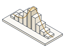
Open the Visualization Workshop and read the summary statistics off two different datasets, and predict — before you read them off the screen — the correlation and regression slope that Anscombe's Set I and Set II share, how far a truncated axis exaggerates a small difference, and how pooling two groups can flip the sign of a trend.
Anscombe's quartet is four datasets with the same mean, variance, correlation and fitted line — yet one is a clean line, one a curve, one a line dragged by a single outlier, and one a vertical stack. The summary statistics cannot tell them apart; only the plot can. A truncated bar axis inflates a small real difference by the exaggeration factor [(v₂−b)/(v₁−b)] ÷ (v₂/v₁), which is 1 only when the baseline is zero. And Simpson's paradox shows a pooled slope reversing every within-group slope. The rule is one sentence: always plot your data.
Open the Visualization Workshop. It has three panels: the Anscombe panel with a set selector, the truncated-axis bar panel with a baseline slider, and the Simpson panel with a group-colour toggle. Each step names the one thing to set; leave the rest.
Anscombe panel  ->  set = I, II, III, IV        Bar panel  ->  baseline slider
Read off  ->  r, slope, intercept, exaggeration factor, pooled vs group slope
Watch the statistics readout for each Anscombe set (mean, variance, r, slope, intercept), the bar panel's exaggeration-factor readout as you drag the baseline, and the Simpson panel's pooled slope beside the two group slopes. Every number you predict is printed there.
In the Anscombe panel, select Set I — a clean linear scatter. Predict the Pearson correlation r, then read the statistics readout.
The readout shows r = 0.816 — a strong positive linear association, exactly as the tidy line looks.
Now select Set II. Its scatter is a clear curve, not a line. Predict its correlation r before you read it — will it differ from Set I?
The readout again shows r = 0.816, identical to Set I to three decimals — yet the shape is a curve. The correlation cannot see the difference; the plot does. This is why you always plot your data.
Stay on Set II and read the regression slope. The OLS slope is b = r·(s_y/s_x). Predict it, then read the slope readout (and note the intercept beside it).
The slope reads 0.5 and the intercept 3 — the very same fitted line as Set I. All four Anscombe sets share the line y = 3 + 0.5x, so not even the regression tells them apart.
Switch to the bar panel: two bars, 100 and 105 — a real difference of 5%. Drag the baseline up to 95 and predict the exaggeration factor, then read it off.
The factor reads about 1.9×: starting the axis at 95 makes the taller bar look nearly twice the other, when the true difference is only 5%. The bars did not change — the axis did.
Keep the same two bars, 100 and 105, and drag the baseline back down to 0. Predict the exaggeration factor now.
The factor is exactly 1.00×: with the axis at zero the visual ratio equals the true ratio, so the chart tells no lie. A zero baseline is the honest default for a bar chart.
Open the Simpson panel. Each of the two groups trends downward with a slope of −1. Turn off the group colouring so the points pool together, and predict the pooled regression slope — up or down?
The pooled slope is +0.714 — it goes up, the opposite of both group slopes of −1. Aggregating across a hidden grouping variable reversed the trend entirely: Simpson's paradox.
Everything above is waiting in the Visualization Workshop. Cycle all four Anscombe sets and watch the summary statistics stay frozen while the pictures change; drag the bar baseline and watch the exaggeration factor climb; and toggle the Simpson grouping to see the pooled line reverse the group lines. Same numbers, different stories — always plot your data.
- Read Anscombe Set I's correlation r = 0.816
- Found Set II sharing the identical r = 0.816 with a completely different, curved scatter
- Confirmed the shared fitted line y = 3 + 0.5x — slope 0.5, intercept 3
- Measured a truncated axis exaggerating a 5% difference by 1.9× at baseline 95, and exactly 1.00× at a zero baseline
- Watched Simpson's pooled slope +0.714 reverse the group slopes of −1
- Every value you predicted is the demo's own arithmetic — proof that summary stats match while pictures differ