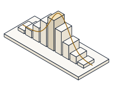
Open the time-series sandbox and take one series apart three ways. Predict — before you read it off the screen — what the autocorrelation at lag 0 must be, where the ACF of a pure seasonal wave spikes, whether a trend + season + noise decomposition adds back to the original series exactly, and what an AR(1) fit's coefficient equals.
A time series is data indexed by time, and it carries memory: today looks like yesterday. The autocorrelation function ρ_k measures that memory at each lag k; it is normalised by the variance, so ρ_0 = 1 for every series, and a seasonal cycle of period P shows up as a spike at lag P. A decomposition splits the series into a slow trend T_t, a repeating season S_t and a residual R_t, defined so that T_t + S_t + R_t = y_t exactly. And an AR(p) model predicts each value from its own past; fit by Yule-Walker, its first coefficient at p = 1 is exactly the lag-1 autocorrelation, φ̂₁ = ρ₁.
Open the sandbox. It opens on its default series (trend slope 0.1, seasonal amplitude 8, period 12, noise SD 2, seed 7, MA window 12, AR order 2). Each step names the sliders to move; press “reset to defaults” between the pure-wave step and the rest.
Sliders  ->  slope / amplitude / period / noise / seed / MA window / AR order p
Defaults ->  0.1 / 8 / 12 / 2 / 7 / 12 / 2      Series: n = 120, level = 50
Watch the readouts: ACF at season, reconstruction (the max of |T+S+R − y|), AR coeffs, and the structure block below (which prints ρ_0, the largest ACF lag, and the p = 1: φ̂ = ρ₁ identity). The series is seeded, so the numbers you predict are exactly the ones printed.
Leave the sandbox on its default series. In the structure block under the plots, the ACF line prints ρ_0 first. Predict its value — the correlation of the series with a copy of itself shifted by 0 steps — then read it.
ρ_0 = 1 — exactly, and for every series. The ACF is the autocovariance divided by the variance γ_0, so at lag 0 the ratio is γ_0 / γ_0 = 1. A series is always perfectly correlated with itself; the interesting question is how fast that correlation decays as the lag grows.
Now build a pure seasonal wave: drag Trend slope to 0 and Noise SD to 0, leaving amplitude 8 and period 12. Predict the ACF at season readout — the autocorrelation at lag 12 — then read it (compare it with the significance band ±0.179).
The ACF at season reads about 0.900 — a tall spike far above the ±0.179 band. A cosine of period 12 repeats every 12 steps, so the series lines up with itself at that lag: seasonality announces itself as a large positive autocorrelation at the seasonal lag.
Stay on the pure wave. The structure block ends with “largest at lag ___”, the lag of the tallest ACF bar beyond lag 0. Predict which lag that is for a wave of period 12, then read it.
The peak sits at lag 12 — the period itself. A sinusoid of period P peaks in its ACF at lag P (and again at 2P, 3P, …). Reading the ACF's dominant lag is how you recover an unknown seasonal period straight from the data.
Press “reset to defaults” to return to the noisy default series. Look at the reconstruction readout — the largest value of |T_t + S_t + R_t − y_t| over the whole series. Predict whether trend + season + residual add back to the original data, then read it.
The reconstruction error is essentially 0 — about 7.1e-15, machine precision. This is not luck: the residual is defined as R_t = y_t − T_t − S_t, so T_t + S_t + R_t = y_t is an identity. The decomposition rearranges the series, it never loses any of it.
Still on the default series, drag AR order p down to 1. The structure block now shows “p = 1: φ̂ = ρ₁ = ___”. Predict the fitted coefficient φ̂₁ and how it relates to the lag-1 autocorrelation, then read it.
The fit gives φ̂₁ ≈ 0.801, and it equals the lag-1 autocorrelation ρ₁ exactly. That is not a coincidence: fitting an AR(1) by Yule-Walker solves φ₁ = γ₁ / γ_0 = ρ₁. The model's one-step memory just is the series' own lag-1 correlation.
Everything above is waiting in the sandbox. Raise the noise and watch the residual grow while the trend and season hold their shape; drop the seasonal amplitude to zero and the ACF spike at lag 12 collapses into the band; push the AR order up and forecast further out to see a stationary model decay back toward the series mean.
- Confirmed ρ_0 = 1 for the series — the ACF is normalised by the variance
- Saw a pure seasonal wave spike to ACF ≈ 0.900 at the seasonal lag, far above the ±0.179 band
- Read the ACF peak at lag 12 — a sinusoid of period P peaks at lag P
- Checked that T + S + R = y to machine precision (≈ 0) — the residual is defined that way
- Fit an AR(1) and found φ̂₁ ≈ 0.801 = ρ₁ exactly — Yule-Walker at p = 1