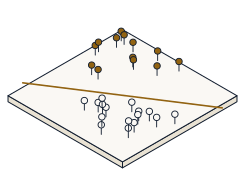
Freeze a pretrained feature map, train a small head on top, and race it against a network trained from scratch in the sandbox — then predict, before you read the panels, the transfer accuracy and the from-scratch accuracy when labels are scarce, confirm the feature map is deterministic, and predict how their gap moves as you hand the models more labels.
A pretrained feature map φ(x) turns raw inputs into features once, and stays frozen; on top of it you fit only a small head — here a ridge-regression probe ŷ = sign(wᵀφ(x) + b₀). Because the head has few parameters, it learns from a handful of labels, so transfer reaches useful accuracy where a network trained from-scratch — which must learn the features and the boundary from the same few labels — still flounders. As labels grow, from-scratch catches up and the gap closes. The feature map here is a synthetic, seeded stand-in — NOT real pretrained weights, and there is no real pretrained model behind it — but every accuracy and the shrinking gap are real, computed numbers.
Open the sandbox. Pick the concentric-circles task, set the label budget with the n slider, and read the transfer, fine-tune and from-scratch accuracy off the panel; the boundary, the sample-efficiency curve and every accuracy update live.
Task -> Concentric circles   Labels n -> 8   Features -> Frozen (transfer)   seed 3/7
Then raise Labels n -> 64, then 256, and watch the gap close
Every number below uses the demo's default seeds (feature seed 3, data seed 7) and its default knobs (gamma = 0.9, H = 40 features), so your panels reproduce them exactly. The feature map is a synthetic stand-in for pretrained weights — the accuracies it enables are real.
Set n = 8 labels on the concentric-circles task and read the transfer model — frozen features with a ridge head. Predict its held-out accuracy before you look.
Transfer scores accuracy = 0.7125. With only eight labels the small head, sitting on the reused features, already separates the rings well above chance.
Now read the from-scratch network at the same n = 8 — it must learn the features and the boundary from those eight labels. Predict its accuracy, and the gap to transfer.
From-scratch scores accuracy = 0.6325, a gap of 0.7125 − 0.6325 = 0.08 below transfer. Too few labels to learn good features from nothing — this is the sample-efficiency win, and exactly why we reuse a pretrained map.
Frozen means fixed: for a given feature seed the map never changes, so the same input always yields the same features. With feature seed 3, gamma = 0.9, H = 40, predict the first activation of φ(x) at x = (0.4, −0.7).
It is exactly φ(x)[0] = -0.996487060176469 (≈ −0.9965), the same value on every run. That reproducibility is the whole point of freezing: the features are computed once and reused, never re-learned.
Raise the budget to n = 64 and watch both models climb. From-scratch now has enough labels to learn real features. Predict the gap accT − accS here (transfer 0.9325 vs from-scratch 0.8825).
The gap has fallen to 0.9325 − 0.8825 = 0.05, down from 0.08 at n = 8. More labels let from-scratch learn the features transfer got for free — so transfer's lead narrows.
Push the budget to n = 256. Both models are near the ceiling now (transfer 0.975, from-scratch 0.96). Predict the gap accT − accS.
The gap is just 0.975 − 0.96 = 0.015 — transfer still leads, but barely. The lesson: transfer's advantage is largest exactly when labels are fewest (0.08 → 0.05 → 0.015 as n climbs). When data is abundant, from-scratch catches up.
Everything above is waiting in the sandbox. Sweep the n slider to watch the sample-efficiency curve — the two accuracy lines start far apart and converge as labels grow — switch the task to moons, spiral or XOR to see the frozen features transfer across shapes, and toggle fine-tune to unfreeze the map. Remember the feature map is a synthetic stand-in, not real pretrained weights — but every accuracy you read is computed.
- Read transfer accuracy = 0.7125 at n = 8 — useful from a handful of labels
- Saw from-scratch trail at accuracy = 0.6325, a 0.08 gap — the sample-efficiency win
- Confirmed the frozen map is deterministic: φ(x)[0] = -0.996487060176469 every run
- Watched the gap shrink as labels grew — 0.08 → 0.05 → 0.015 at n = 8, 64, 256
- Every accuracy and gap you predicted is the demo's own real ridge, gradient-descent and sample-efficiency arithmetic — only the frozen feature map is a synthetic stand-in, not real pretrained weights