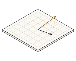
Measure a matrix's condition number, test when an iterative solver converges, and watch a near-singular system amplify a perturbation in the sandbox, and predict — before you read it off the screen — that κ is exactly one for a perfectly-scaled matrix and large for a stretched one, that the Jacobi iteration converges precisely when its spectral radius ρ is below one, and that an ill-conditioned system blows a tiny input error up by a factor of κ.
The condition number κ(A) = σmax/σmin is the ratio of the largest to the smallest singular value — the real σmax/σmin, not a shortcut from column norms. It says how much a matrix can stretch relative to how much it can squash: κ = 1 is perfectly conditioned, a huge κ is nearly singular. For the iterative solvers, Jacobi and Gauss-Seidel converge iff the spectral radius of the iteration matrix — its largest eigenvalue magnitude ρ = maxi|λi| — is below one, which strict diagonal dominance guarantees. And the two ideas meet in the error bound ‖δx‖/‖x‖ ≤ κ(A)·‖δb‖/‖b‖: the condition number is exactly the worst-case factor by which a relative input error is amplified.
Open the sandbox. It reports a matrix's singular values and condition number, runs Jacobi and Gauss-Seidel on A x = b with a convergence verdict, and perturbs b to measure the amplification. Each step names the matrix to set, then read the κ, the spectral radius, the verdict and the amplification readouts.
Condition:  A = I = [[1,0],[0,1]]     and     A = diag(1,100) = [[1,0],[0,100]]
Iterate:  [[4,1],[1,3]] b=(1,2)  vs  [[1,3],[2,1]] b=(4,3)     Amplify:  [[1,1],[1,1.0001]] b=(2,2.0001), perturb b by 0.001
Watch the condition-number readout κ, the Jacobi spectral radius ρ and converges/diverges verdict, and the error-amplification ratio — every number you predict is printed there.
Set A = I, the identity [[1,0],[0,1]]. Both singular values are 1, so κ = σmax/σmin. Predict κ, then read the condition-number readout.
The condition number is κ = 1: the identity neither stretches nor squashes, so its largest and smallest singular values are equal. A well-conditioned matrix passes relative errors through unchanged — it is the best case there is.
Set A = diag(1, 100) = [[1,0],[0,100]] — it scales one axis by 1 and the other by 100. The singular values are σmax = 100 and σmin = 1. Predict κ = σmax/σmin, then read it.
The condition number is κ = 100: exactly σmax/σmin = 100/1, the real ratio of singular values — not a proxy from column norms, which can be off by orders of magnitude. This matrix magnifies a relative input error up to a hundredfold.
In the iterative panel set A = [[4,1],[1,3]], b = (1, 2) and run Jacobi. Its iteration matrix has spectral radius ρ = maxi|λi|. Predict roughly whether ρ is below 1, then read the spectral-radius readout.
The spectral radius is ρ ≈ 0.289 — well below 1. Because the diagonal entries dominate the off-diagonal ones, the iteration matrix has small eigenvalues, so each Jacobi sweep shrinks the error by roughly 0.289.
Keep A = [[4,1],[1,3]], b = (1, 2). The convergence rule is exactly ρ < 1. Predict the verdict (1 = converges, 0 = diverges), then read it.
The verdict is 1: it converges, because ρ ≈ 0.289 < 1. Strict diagonal dominance is a sufficient condition for exactly this — the errors of successive iterates form a shrinking geometric sequence governed by ρ.
Now set the non-dominant A = [[1,3],[2,1]], b = (4, 3) — the off-diagonal entries (3 and 2) exceed the diagonal ones. Predict the Jacobi spectral radius ρ, then read it.
The spectral radius is ρ ≈ 2.449 — above 1, so Jacobi diverges: the residual grows each sweep instead of shrinking. Diagonal dominance is what separates the two regimes; lose it and the same iteration that converged now runs away.
In the amplification panel set the near-singular A = [[1,1],[1,1.0001]], b = (2, 2.0001), and perturb b by a relative 0.001 (0.1%). Its condition number is about 40002. Predict the amplification ratio (‖δx‖/‖x‖) / (‖δb‖/‖b‖), then read it.
The ratio is about 40002 — a 0.1% nudge to b becomes a roughly 4000% error in the solution. That factor is exactly the condition number κ, the worst-case ceiling of the bound ‖δx‖/‖x‖ ≤ κ·‖δb‖/‖b‖. This is why conditioning, not just correctness of the algorithm, decides the accuracy.
Everything above is waiting in the sandbox. Change the matrix and watch the singular values, the condition number and the unit-circle-to-ellipse image respond; run Jacobi and Gauss-Seidel and see the residual trace converge or diverge as the spectral radius crosses one; and dial the perturbation to watch a well-conditioned system shrug it off while a near-singular one blows it up.
- Measured κ(I) = 1 — a perfectly-conditioned matrix
- Measured κ(diag(1,100)) = 100, the real σmax/σmin, not a proxy
- Read the Jacobi spectral radius ρ ≈ 0.289 for [[4,1],[1,3]]
- Confirmed ρ < 1 gives the verdict 1 — it converges
- Saw the non-dominant [[1,3],[2,1]] reach ρ ≈ 2.449 > 1 — it diverges
- Watched a near-singular system amplify a 0.1% perturbation by 40002 = κ
- Every value you predicted is the demo's own numerical arithmetic, not a picture