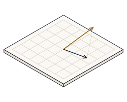
Orthonormalise vectors with Gram-Schmidt, project a target onto a subspace, and fit a line by least squares in the sandbox, and predict — before you read it off the screen — that Gram-Schmidt returns perpendicular unit vectors, that a projection's residual is orthogonal to the subspace, and that least squares recovers a line exactly through collinear points.
Two vectors are orthogonal when their dot product is zero. Gram-Schmidt turns any independent set into an orthonormal basis q₁, q₂, … — perpendicular and each of length one — by subtracting from each vector its projection onto every basis vector already accepted, then normalising. Projecting a target b onto that subspace gives proj = ∑ᵢ (b · qᵢ) qᵢ; the leftover residual = b − proj is always ⊥ to the subspace. Least squares is the same idea: the best-fit line projects b onto the column space of A, solving the normal equations AᵀA x̂ = Aᵀb.
Open the sandbox. The Gram-Schmidt panel takes two vectors v₁, v₂; the projection panel projects a target b onto a chosen subspace; the least-squares panel fits a line to a dataset. Each step names the values to set, then read the orthonormal basis, the projection, the residual and the fit readouts.
Gram-Schmidt:  v1 = (2, 1),  v2 = (1, 3)   |   Project b = (2, 3) onto span{(1, 0)}
Least squares:  xs = 0 1 2 3 4,  ys = 1 3 5 7 9   (Read: q1.q2, |q1|, proj, residual, slope, RMS)
Watch the orthonormality check (q₁ · q₂ and each |qᵢ|), the projection and residual readouts, and the least-squares slope and RMS — every number you predict is printed there.
Set v₁ = (2, 1) and v₂ = (1, 3) — independent. Gram-Schmidt keeps q₁ along v₁, then subtracts v₂'s component along q₁. Predict the dot product q₁ · q₂, then read the readout.
The dot product is q₁ · q₂ = 0: the two basis vectors are orthogonal. Removing v₂'s q₁ component leaves a remainder perpendicular to q₁ by construction.
Keep v₁ = (2, 1), v₂ = (1, 3). After orthogonalising, Gram-Schmidt divides each remainder by its own length. Predict |q₁|, then read the length readout.
The length is |q₁| = 1. "Orthonormal" means both perpendicular and normalised — dividing by |w| is the step that makes each vector exactly one unit long.
In the projection panel set the target b = (2, 3) and project it onto the x-axis, span{(1, 0)}. Predict the x-component of the projection proj, then read the readout.
The projection is proj = (2, 0), so its x-component is 2: projecting onto the x-axis keeps the horizontal part of b and discards the vertical part — the coefficient is b · q₁ = 2.
Keep b = (2, 3) projected onto span{(1, 0)}. The residual is residual = b − proj = (0, 3). Predict its dot product with q₁, then read the readout.
The dot product is residual · q₁ = 0: the leftover is ⊥ to the subspace. That is what makes the projection the closest point in the subspace to b — nothing is left pointing along it.
In the least-squares panel choose the exactly-collinear dataset xs = 0 1 2 3 4, ys = 1 3 5 7 9 — the points lie on y = 1 + 2x. Predict the fitted slope c₁, then read it.
The slope is c₁ = 2 (and the intercept c₀ = 1): the normal equations AᵀA x̂ = Aᵀb recover the exact line when the points already lie on one.
Keep the collinear dataset xs = 0 1 2 3 4, ys = 1 3 5 7 9. The fitted line passes through every point. Predict the RMS residual RMS, then read it.
The error is RMS = 0: every residual is zero, so the projection of b onto the column space is b itself. Pull one point off the line (try the outlier dataset) and the RMS jumps above zero.
Everything above is waiting in the sandbox. Drag the vectors and watch Gram-Schmidt orthonormalise them step by step, move the target and see its projection and residual update, and swap datasets to watch the least-squares line and its RMS respond — then check that the residual stays perpendicular however you push things around.
- Orthonormalised (2, 1) and (1, 3) with Gram-Schmidt — perpendicular, q₁ · q₂ = 0
- Confirmed each basis vector has unit length, |q₁| = 1
- Projected b = (2, 3) onto the x-axis — proj = (2, 0)
- Saw the residual (0, 3) is orthogonal to the subspace, residual · q₁ = 0
- Fit the collinear line by least squares — slope c₁ = 2, RMS = 0
- Every value you predicted is the demo's own orthogonality arithmetic, not a picture