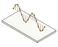
Run the matched filter on a signal buried in noise in the sandbox, and predict — before you read it off the screen — the energy its correlation peak reaches, the area under the ROC when the signal is detectable and when it is not, and the processing gain a longer template buys.
A matched filter is the optimal detector in white noise: it cross-correlates the record with the known template, so the signal adds up in phase while the noise does not. Its peak stands 10·log10(N) dB above where a single sample sat — the processing gain — and the ROC turns that margin into a P_d-versus-P_fa trade you can read. Predicting the peak energy, the AUC and the gain off a real run is how detection stops being a black box.
Open the sandbox. It opens on exactly this state — a chirp template buried in unit-variance noise — so a Reset gets you here too. Each step names the one knob to change; leave everything else alone.
Template  ->  Chirp      N  ->  64        A  ->  0.30
Noise sigma  ->  1.00     Threshold  ->  2.00 sigma_out     Seed  ->  7
Watch the template-energy readout, the AUC readout and the correlation peak — every number you predict is printed there.
Keep the defaults: a Chirp template of N = 64 samples. The matched filter cross-correlates the record with the template; matched against itself (autocorrelation) it peaks at zero lag with value E_s = Σs². Every template here is normalised so E_s = N. Predict it, then read the template-energy readout.
The template energy is E_s = Σs² = N = 64, and the noiseless autocorrelation peaks at exactly that value at lag 0 — the matched filter's defining property.
Keep the defaults: A = 0.30, N = 64, sigma = 1, so the detectability is d = A·√N / sigma = 2.4. Sweep the threshold and read the area under the ROC. Predict whether the AUC sits near 0.5 (chance) or near 1, then read the AUC readout.
The ROC bows toward the top-left and the AUC ≈ 0.955 — well above the 0.5 of chance. At d = 2.4 the buried signal is comfortably detectable.
Drag the amplitude A down to 0. With no signal, P_d = Q((tau − 0)/sigma) = Q(tau/sigma) = P_fa at every threshold. Predict the AUC, then read it.
The ROC collapses to the diagonal and the AUC = 1/2 = 0.5 — pure chance. At tau = 0 both P_fa and P_d equal Q(0) = 0.5.
Drag the template length N up to 100. Coherent integration over N samples multiplies the output power SNR by N — a gain of 10·log10(N), independent of the signal amplitude. Predict the processing-gain readout.
The processing gain is 10·log10(100) = 20 dB — a hundredfold power advantage the matched filter buys purely from template length (the default N = 64 gives 18.06 dB).
Everything above is waiting in the sandbox. Bury the template deeper by lowering the amplitude or raising the noise, sweep the threshold to walk the whole ROC, lengthen the template to watch the gain climb, and switch on the Monte-Carlo overlay to see thousands of seeded draws converge onto the analytic curve.
- Read the matched filter peaking at its energy, E_s = Σs² = N = 64
- Watched a buried signal (d = 2.4) bow the ROC to an AUC ≈ 0.955
- Saw the ROC collapse to the diagonal (AUC = 0.5) when the signal went to zero — pure chance
- Found the processing gain of an N = 100 template, 10·log10(100) = 20 dB
- Every value you predicted is the demo's own detection arithmetic, not a picture